PGI-15 Tutorial

Artificial Neural Networks

02.11.2023 | Emre Neftci, Susanne Kunkel, Jamie Lohoff, and Willem Wybo

The First Artificial Neuron

In 1943, Warren McCulloch and Walter Pitts propose the first artificial neuron, the Linear Threshold Unit.
$f$ is a step function: $$ y = \begin{cases} f(a) &= 1\text{ if } \ge 0\\ f(a) &= 0\text{ if } a< 0\\ \end{cases} $$
$a$ is a weighted sum of inputs $x$
"Modern" artificial neurons are similar, but $f$ is typically a sigmoid or rectified linear function

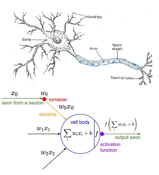
Mathematical Model of the Artificial Neuron

$x_i$ is the state of the input neurons
$w_i$ is the weight of the connection
$b$ is a bias
The total input to the neuron is: $ a = \sum_i w_i x_i +b $
The output of the neuron is: $ y = f(a) $
where $f$ is the activation function

The Perceptron

The Perceptron is a special case of the artificial neuron where: \[ \begin{eqnarray} \mbox{y} & = & \begin{cases} -1 & \mbox{if } a = \sum_j w_j x_j + b \leq 0 \\\\ 1 & \mbox{if } a = \sum_j w_j x_j + b > 0 \end{cases} \end{eqnarray} \]
Three inputs $x_1$, $x_2$, $x_3$ with weights $w_1$, $w_2$, $w_3$, and bias $b$

Perceptron Example

Like McCulloch and Pitts neurons, Perceptrons can be hand-constructed to solve simple logical tasks
Let's build a "sprinkler" that activates only if it is dry and sunny.
Let's assume we have a dryness detector $x_0$ and a light detector $x_1$ (two inputs)
Find $w_0$, $w_1$ and $b$ such that output $y$ matches target $t$

Sunny	Dry	$t$
1 (yes)	1 (yes)	1
1 (yes)	0 (no)	0
0 (no)	1 (yes)	0
0 (no)	0 (no)	0

$w_0 =$ 0	$w_1 =$ 0	$b =$ 0

Logic Gates

Logic gates are (idealized) devices that perform one logical operation
Common operations are AND, Not, and OR and can perform Boolean logic
Using only Not AND (NAND) gates, any boolean function can be built.

Linear separability

A perceptron is equivalent to a decision boundary.

A straight line can separate blue vs. red

There is no straight line that can separate blue vs. red

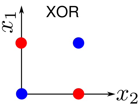
Problems where a straight line can separate two classes are called Linearly Separable

Perceptron learning algorithm to learn to classify linearly separable points

Optimization Algorithm Gradient Descent

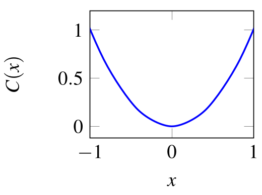
Example: Find $x$ that minimizes $C(x) = x^2$
Incremental change in $\Delta x$: $$ \begin{eqnarray} \Delta C \approx \underbrace{\frac{\partial C}{\partial x}}_{\text{=Slope of }C(x)} \Delta x \end{eqnarray} $$ Gradient Descent rule: $\Delta x = - \eta \frac{\partial C}{\partial x}$, $\Delta C \approx - \eta \left( \frac{\partial C}{\partial x} \right)^2$
Gradient Descent for finding the optimal $x$: $ \begin{eqnarray} x \leftarrow x - \eta \frac{\partial C}{\partial x} \end{eqnarray} $

Linear separability

A perceptron is equivalent to a decision boundary.

A straight line can separate blue vs. red

There is no straight line that can separate blue vs. red

Problems where a straight line can separate two classes are called Linearly Separable

Most complex problems are not linearly separable

Deep neural networks

How many hidden layers and how many units per layer do we need? The answer is at most two

Hertz, et al. 1991

Szegedy et al. 2014

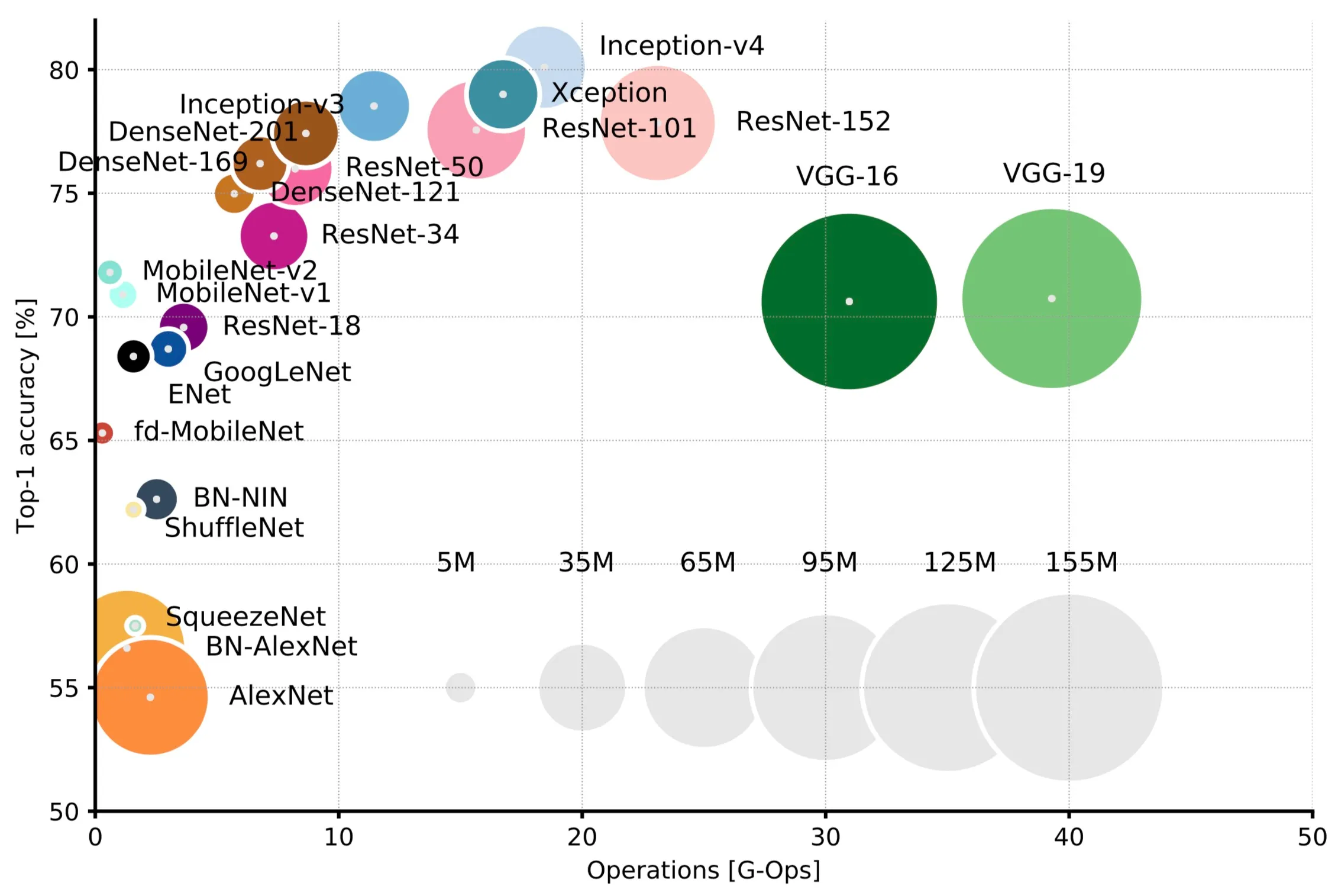
Canziani et al. 2018

Single Layer Network with Sigmoid Units M

Weight matrix: $W^{(1)} \in \mathbb{R}^{N\times M}$ (meaning $M$ inputs, $N$ outputs) $$ \begin{eqnarray} y^{(1)}_i &=& \sigma(\underbrace{\sum_j W^{(1)}_{ij} x_j}_{a_i^{(1)}}) \\ \end{eqnarray} $$
MSE cost function, assuming a single data sample $\mathbf{x}\in\mathbb{R}^{M} $, and target vector $\mathbf{t}\in\mathbb{R}^{N}$ $$ C_{MSE} = \frac{1}{2} \sum_i(y^{(1)}_i - t_i)^2 $$
Gradient w.r.t. $W^{(1)}$ (in scalar form): $$ \frac{\partial }{\partial W^{(1)}_{ij}} C_\text{MSE}= (y^{(1)}_i - t_i) \sigma'(a^{(1)}_i) x_j $$

## Single Layer Network with Sigmoid Units

<p> Neural networks operations are generally written in Matrix form</p>

<div class=row>
        <div class=column>
          <center>Scalar Form (one sample)</center>
        $$
        \begin{split}
        a_i^{(1)} &= \sum_j W^{(1)}_{ij} x_j, \quad y^{(1)}_i = \sigma(a_i^{(1)}) \\
        \delta_i^{(1)} &= \frac{1}{N^{s}} (y^{(1)}_i - t_i) \sigma'(a^{(1)}_i)\\
        \Delta W_{ij} &=  -\eta \delta_i x_j
        \end{split}
        $$
        </div>
        <div class=column>
          <center>Matrix Form ($N^{s}$ samples)</center>
          <div class=fragment>
          $$
          \begin{split}
          A^{(1)} & = X W^{(1),T}, \quad 
          Y^{(1)}  = \sigma(A^{(1)}) \\ 
          \end{split}
          $$
          </div>
          <div class=fragment>
          $$
          \begin{split}
          \delta &= \frac{1}{N^{s}} (Y^{(1)} - T) \odot \sigma'(A^{(1)}) \\
          \end{split}
          $$
          </div>
        <div class=fragment>
        $$
        \begin{split}
        \Delta W & =  - \eta \delta^T \mathbf{X} \\
        \end{split}
        $$
        </div>
        </div>
        </div>
        $$
        W \leftarrow W + \Delta W 
        $$
        <ul>
          <li /> $\delta$ $\in \mathbb{R}^{N^{s}\times N}$, $X$ $\in \mathbb{R}^{N^{s} \times M}$, and dimension of $\Delta W$ must be same as $W$!
        </ul>

[![Open In Colab](https://colab.research.google.com/assets/colab-badge.svg)](https://drive.google.com/file/d/1JWYVKVvxvdKnwEepO3_fnw4Vq-CJ2ysy/view?usp=sharing)

Two Layer Network with Sigmoid Units

Two layers means we have two weight matrices $W^{(1)}$ and $W^{(2)}$
$W^{(1)} \in \mathbb{R}^{N^{(1)}\times M}$, $W^{(2)} \in \mathbb{R}^{N^{(2)}\times N^{(1)}}$
The output is a composition of two functions:

$$ \begin{eqnarray} \mathbf{y}^{(1)} &=& \sigma(W^{(1)} \mathbf{x} ) \\\\ \mathbf{y}^{(2)} &=& \sigma(W^{(2)} \mathbf{y}^{(1)} ) \\\\ \end{eqnarray} $$

Cost function $ C_{MSE} = \sum_{i=1}^{N^{(2)}}(y^{(2)}_i - t_i)^2 $
Gradient wrt $W^{(2)}$ is: $ \frac{\partial }{\partial W^{(2)}_{ij}} C_\text{MSE}= \underbrace{(y^{(2)}_i - t_i) \sigma'(a^{(2)}_i)}_{\delta^{(2)}_i} y^{(1)}_j $
Gradient wrt $W^{(1)}$ is: $ \frac{\partial}{\partial { W_{jk}^{(1)}}} C_{\text{MSE}} = \underbrace{(\sum_i \delta_i^{(2)} W^{(2)}_{ij}) \sigma'(a^{(1)}_j)}_{\text{backpropagated error}\, \delta^{(1)}_{j}} x_k $
This is a special case of the gradient backpropagation algorithm

<div style='font-size:24px;text-align:left;' >
          <p>The task of learning is to minimize a cost function $\mathcal{L}$ over the entire dataset.
        In a neural network, this can be achieved by gradient descent, which modifies the network parameters $\mathbf{W}$ in the direction opposite to the gradient:
        $$
        \begin{split}
          W_{ij} \leftarrow W_{ij} - \eta \Delta W_{ij},  & \text{where } \Delta W_{ij} =
         \frac{\partial \mathcal{L}}{\partial W_{ij}} =
         \frac{\partial \mathcal{L}}{\partial y_i} 
         \frac{\partial y_i}        {\partial  a_i }       
         \frac{\partial a_i}        {\partial W_{ij}}      
        \end{split}
        $$
        with $a_i = \sum_j W_{ij} x_j$ the total input to the neuron, $y_i$ is the output of neuron $i$, and $\eta$ a small learning rate.
        The first term is the error of neuron $i$ and the second term reflects the sensitivity of the neuron output to changes in the parameter.
        In multilayer networks, gradient descent is expressed as the BP of the errors starting from the prediction (output) layer to the inputs.
        Using superscripts $l=0,...,L$ to denote the layer ($0$ is input, $L$ is output):

`$$
        \frac{\mathrm{\partial}}{\mathrm{\partial} W^{(l)}_{ij}} \mathcal{L} =
        \delta_{i}^{(l)} y^{(l-1)}_j,\text{ where }\delta_{i}^{(l)} = \sigma'\left(
        a_i^{(l)} \right) \sum_k \delta_{k}^{(l+1)} W_{ik}^{\top,(l)},
        $$`

where $\sigma'$ is the derivative of the activation function, and $\delta_{i}^{(L)}=\frac{\partial \mathcal{L}}{\partial y_i^{(L)}}$ is the error of
        output neuron $i$ and $y_{i}^{(0)}=x_i$ and $\top$ indicates the transpose.
        </p>
        </div>

End

Lecture 3: Recurrent Neural Networks Lecture 4: Learning and Plasticity

INPUT		OUTPUT
A	B	A NAND B
0	0	1
0	1	1
1	0	1
1	1	0